Novel Fetal Hemoglobin Modifying Loci Revealed with Genome Wide Studies of Sickle Cell Disease Patients from Cameroon, and Global Metanalysis
Content
- Load required r package
- Clinical datasets
- Summary of Cameroon data
- Summary of Tanzania data
- HbF normalization
- HbF distribution before and after normalization
Load require r package
library(tidyverse)
Clinical datasets
cm <- read_table("../clinicaldata/cm_clinical_data.tsv")
tz <- read_table("../clinicaldata/tz_clinical_data.tsv")
Summary of Cameroon data
Variables
cm %>% names()

##  [1] "FID"                 "IID"                 "AGE"
##  [4] "SEX"                 "HbF"                 "HbS"
##  [7] "Hb_Phenotype"        "Hb"                  "Phenotypes"
## [10] "Genotypes"           "Haplotypes"          "athal"
## [13] "Curated_Age_yrs"     "VOC.year"            "Consultation.year"
## [16] "Hosp"                "Stroke"              "HbA2_percentage"
## [19] "RBC"                 "MCV.fl."             "MCHC"
## [22] "WBC"                 "Lymp"                "Mono"
## [25] "Platelets"           "Curated_penotype"    "Sample_name_comment"
Summary statistics
Quantitative/Continuous variables
variables <- c(
  "AGE",                   # Age in years
  "HbS",                   # Proportion of HbS
  "HbF",                   # Proportion of fetal haemoglobin
  "HbA2_percentage",       # Proportion of HbA2
  "Consultation.year",     # Number of consultations per year
  "MCHC",                  # Mean corpuscular haemoglobin concentration
  "Mono",                  # Monocyte count (x10^9/l)
  "Hosp",                  # Number of hospitalizations per year
  "RBC",                   # Red blood cell count (x10^12/l)
  "WBC",                   # White blood cell count (x10^9/l)
  "Platelets",             # Platelet count (x10^9/l)
  "VOC.year",              # Number of vaso occlusive crises per year
  "MCV.fl.",               # Mean cell volume
  "Lymp"                   # Lymphocyte count (x10^9/l)
)
cm %>%
  select(variables) %>%
  summary()

##       AGE             HbS             HbF         HbA2_percentage
##  Min.   : 5.00   Min.   :19.60   Min.   : 0.700   Min.   : 0.000
##  1st Qu.:10.00   1st Qu.:80.30   1st Qu.: 4.700   1st Qu.: 2.700
##  Median :16.00   Median :86.00   Median : 8.500   Median : 3.200
##  Mean   :18.05   Mean   :83.56   Mean   : 9.892   Mean   : 3.324
##  3rd Qu.:24.00   3rd Qu.:90.70   3rd Qu.:13.600   3rd Qu.: 3.800
##  Max.   :66.00   Max.   :96.50   Max.   :37.400   Max.   :18.200
##                                                   NA's   :3
##  Consultation.year      MCHC            Mono            Hosp
##  Min.   : 0.000    Min.   : 3.80   Min.   :0.000   Min.   : 0.000
##  1st Qu.: 0.000    1st Qu.:25.90   1st Qu.:0.700   1st Qu.: 1.000
##  Median : 1.000    Median :31.00   Median :1.000   Median : 1.000
##  Mean   : 2.049    Mean   :29.21   Mean   :1.161   Mean   : 1.974
##  3rd Qu.: 2.000    3rd Qu.:33.00   3rd Qu.:1.400   3rd Qu.: 2.000
##  Max.   :15.000    Max.   :54.20   Max.   :9.400   Max.   :24.000
##  NA's   :805       NA's   :17      NA's   :14      NA's   :59
##       RBC            WBC           Platelets         VOC.year
##  Min.   :0.84   Min.   : 0.400   Min.   :  22.0   Min.   : 0.000
##  1st Qu.:2.29   1st Qu.: 8.607   1st Qu.: 310.0   1st Qu.: 1.000
##  Median :2.70   Median :11.200   Median : 401.0   Median : 2.000
##  Mean   :2.75   Mean   :11.819   Mean   : 415.4   Mean   : 3.189
##  3rd Qu.:3.12   3rd Qu.:14.200   3rd Qu.: 498.0   3rd Qu.: 4.000
##  Max.   :7.70   Max.   :49.800   Max.   :1185.0   Max.   :48.000
##  NA's   :15     NA's   :14       NA's   :13       NA's   :29
##     MCV.fl.           Lymp
##  Min.   : 59.0   Min.   : 0.100
##  1st Qu.: 81.0   1st Qu.: 3.570
##  Median : 87.0   Median : 4.700
##  Mean   : 87.1   Mean   : 5.186
##  3rd Qu.: 94.0   3rd Qu.: 6.210
##  Max.   :132.0   Max.   :22.600
##  NA's   :14      NA's   :13
Categorigal variables
cm %>%
  select(SEX) %>%
  table() %>%
  as.data.frame() %>%
  na.omit() %>%
  mutate(Prop = (Freq/sum(Freq))*100) -> sex       # Sex

sex

##   . Freq  Prop
## 1 F  657 52.56
## 2 M  593 47.44

colnames(sex) <- c(
  "cat",
  "freq",
  "prop"
)

par(
  mar = c(4,4,3,4)
)

barplot(
  sex$prop,
  ylim = c(0, 60),
  col = c(2,4)
)

text(
  x = c(0.7,1.9),
  y = 30,
  labels = c("Female", "Male")
)

mtext(
  text = "Proportion (%)",
  side = 2,
  line = 3
)

mtext(
  text = "Sex",
  side = 1,
  line = 1
)
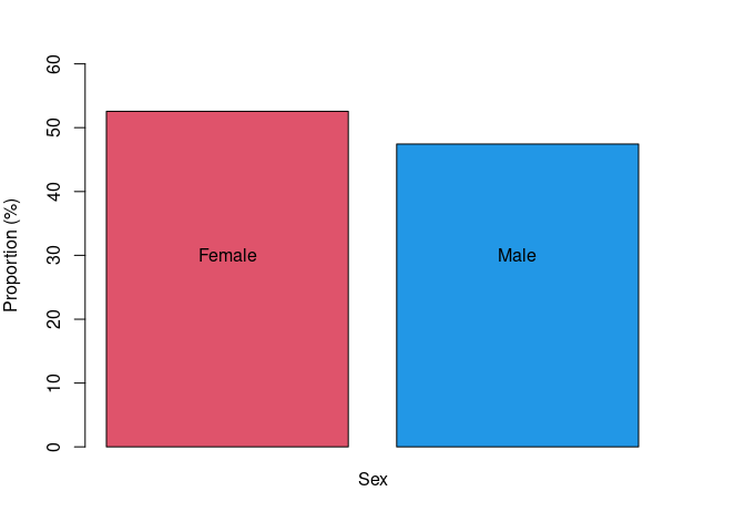
Figue 1. Proportion of females and males in the discovery dataset of Cameroonian inidividuals
# Number of patients with at least one overt stroke
cm %>%
  select(Stroke) %>%
  table()

## .
##   No  Yes
## 1195   46

# 3.7 kb HbA1/HbA2 alpha thalassaemia deletion
cm %>%
  select(athal) %>%
  table()

## .
## α3.7/α3.7   αα/α3.7     αα/αα
##        18       101       286

# HBB gene cluster haplotypes
cm %>%
  select(Haplotypes) %>%
  table()

## .
##     Atypical          BEN       BEN/AI BEN/Atypical      BEN/CAM      BEN/CAR
##            3          331            2           26           99            2
##          CAM       CAM/AI CAM/Atypical      CAM/SEN          CAR CAR/Atypical
##          174            1            8            1            1            1
##      CAR/CAM          SEN
##            1            4
CAM = CAM/CAM, BEN = BEN/BEN, SEN = SEN/SEN, CAR = CAR/CAR, Atypical = Atypical/Atypical
Summary of Tanzania data
Variables
tz %>% names()

## [1] "FID" "IID" "AGE" "HbF" "SEX"
Summary statistics
Quantitative/Continuous variables
variables <- c(
  "AGE",
  "HbF"
)

tz %>%
  select(variables) %>%
  summary()

##       AGE              HbF
##  Min.   : 5.021   Min.   : 0.200
##  1st Qu.: 7.876   1st Qu.: 2.600
##  Median :11.069   Median : 4.800
##  Mean   :13.288   Mean   : 5.748
##  3rd Qu.:16.298   3rd Qu.: 7.800
##  Max.   :44.310   Max.   :32.500
Categorical variable
tz %>%
  mutate(sex.updated = ifelse(SEX == 1, "M", ifelse(SEX == 2, "F", NA))) %>%
  select(sex.updated) %>%
  table() %>%
  as.data.frame() %>%
  na.omit() %>%
  mutate(Prop = (Freq/sum(Freq))*100) -> sex           # Sex

sex

##   . Freq   Prop
## 1 F  539 52.895
## 2 M  480 47.105

colnames(sex) <- c(
  "cat",
  "freq",
  "prop"
)

par(
  mar = c(4,4,3,4)
)

barplot(
  sex$prop,
  ylim = c(0, 60),
  col = c(2,4)
)

text(
  x = c(0.7,1.9),
  y = 30,
  labels = c("Female", "Male")
)

mtext(
  text = "Proportion (%)",
  side = 2,
  line = 3
)

mtext(
  text = "Sex",
  side = 1,
  line = 1
)

Figure 2. Proportion of females and males in the replication dataset of Tanzanian inidividuals
HbF normalization (Cubic root)
Cameroon
cm %>%
  mutate(normalizedHbF = HbF^(1/3)) -> cm.hbf.norm

write.table(
  cm.hbf.norm,
  "../clinicaldata/cm_clinical_data_updated.tsv",
  col.names = T,
  row.names = F,
  quote = F,
  sep = "\t"
)

cm.hbf.norm %>%
  select(HbF, normalizedHbF) %>%
  head()

## # A tibble: 6 × 2
##     HbF normalizedHbF
##   <dbl>         <dbl>
## 1  31.6          3.16
## 2   6.4          1.86
## 3  12.6          2.33
## 4   8.8          2.06
## 5  17.5          2.60
## 6  17.8          2.61
Tanzania
# Tanzania
tz %>%
  mutate(normalizedHbF = HbF^(1/3)) -> tz.hbf.norm

write.table(
  tz.hbf.norm,
  "../clinicaldata/tz_clinical_data_updated.tsv",
  col.names = T,
  row.names = F,
  quote = F,
  sep = "\t"
)

tz.hbf.norm %>%
   select(HbF, normalizedHbF) %>%
   head()

## # A tibble: 6 × 2
##     HbF normalizedHbF
##   <dbl>         <dbl>
## 1   0.2          0.585
## 2   0.3          0.669
## 3   0.3          0.669
## 4   0.3          0.669
## 5   0.3          0.669
## 6   0.4          0.737
HbF distribution before and after normalization
cm.hbf.den <- density(
  cm.hbf.norm$HbF
)

cm.nhbf.den <- density(
  cm.hbf.norm$normalizedHbF
)

tz.hbf.den <- density(
  tz.hbf.norm$HbF
)

tz.nhbf.den <- density(
  tz.hbf.norm$normalizedHbF
)

par(
  mar = c(4,4,3,4)
)

plot(
  cm.hbf.den,
  main = "Cameroon HbF"
)

polygon(
  cm.hbf.den,
  col = 2
)

plot(
  cm.nhbf.den,
  ylab = "",
  main = "Cameroon normalized HbF"
)

polygon(
  cm.nhbf.den,
  col=5
)

plot(
  tz.hbf.den,
  main = "Tanzania HbF"
)

polygon(
  tz.hbf.den,
  col = 2
)

plot(
  tz.nhbf.den,
  ylab = "",
  main = "Tanzania normalized HbF"
)

polygon(
  tz.nhbf.den,
  col = 5
)

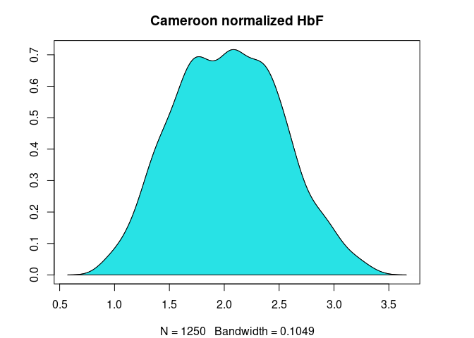
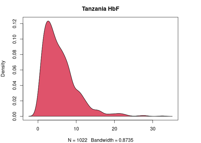
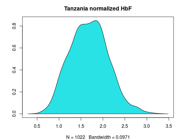
Figure 3. HbF distribution in Cameroonian and Tanzanian study participants before and after normalization